Discrete event simulation using spreadsheets — a case in Healthcare operations.
Discrete event simulation (DES) is a very useful way of representing processes that can be separated into distinct “events” that interact over time. Spreadsheets can be a simple and widely available way to simulate DES to obtain information for decision making. Spreadsheets are a great tool for visualizing data about a process because they store information in tabular form.
In this article, I will describe a way of representing DES in spreadsheets for healthcare delivery. Before discussing how to deal with distributions in Excel, I will first describe the case. Finally, I describe the spreadsheet and its results.
An example google sheets speadsheet of this simulation can be found here.
Case Description
Let us consider a process where a patient arrives at a healthcare facility, is first seen by a nurse, then seen by a physician, and is thereafter released from the facility.

Some characteristics of this process are:
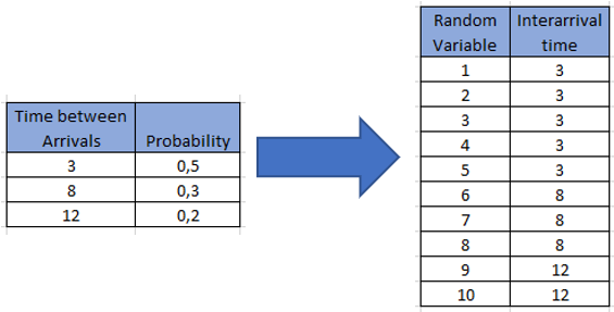
- - The arrival of patients varies over time, but from past history it has been determined that 50% of the time patients arrive about 3 minutes after the previous patient, 30% of the time this time between arrivals is about 8 minutes, and the rest of the time is about 12 minutes between the arrival of each patient.

2. The time each nurse needs to check up on patients is quite standard, as the procedures are well established (for example, measuring blood pressure, patient temperature, and weight and height), and this usually takes 7 minutes for every patient.
3. The amount of time each physician needs to check on patients is variable, depending on the problems discovered by the nurse or any specific ailments disclosed by the patient. From past history, it has been found that 30% of the time the physician spends about 8 minutes with the patient, 50% of the time the physician spends about 12 minutes with the patient, and the rest of the time (about 20% of the time), this attention time is 17 minutes.
Dealing with discrete distributions
When describing, for example, the time between the arrival of patients, I mentioned past data in terms of the probabilities associated with certain values for these times in the past. Despite this, we have no idea what interarrival time the next patient will have.
All we know is that this inter-arrival time could be 3 minutes with 50% probability, 8 minutes with 30% probability, or 12 minutes with 20% probability.
We call this a random variable with a discrete probability distribution (it is not continuous as it can only take some specific values. One way of using this in practice is to:
- Consider the numbers 1 to 10, and assign to these numbers the interarrival time values according to their probabilities. For example, 50% of the values, say 1 to 5, will have the value 3, for 30% of the values, say 6 to 8, the interarrival time value is 8, and finally for the last 20% of the values, say 9 and 10, the interarrival time value is 12. 2)
- When a new patient arrives, we choose at random a value from 1 to 10, and then use the corresponding interarrival time value for that specific patient.
The same process can be followed to determine the service time for physicians.
Simulating the process
The simulation process is centered around patients. Every row in the spreadsheet represents a patient in sequentiual order of arrival. Since the shift starts at 7:00 AM, we find that the next arrival corresponds to the random variable 6, which maps to an interarrival time of 8 minutes through a VLOOKUP function:
=VLOOKUP(H13;Patient!$B$3:$C$12;2;FALSE)
This arrival therefore happens at 7:08 AM. This is the calculation process with subsequent patients.

Service finish times are the sum of the service start time and the service time, fixed in the case of the nurses and a discrete probability distribution in the case of the physicians. Waiting times are the difference between the service start time and either the arrival time (in case of the waiting times for nurse checkup) or the nurse checkup service finish time (in case of witing times for the physician checkup).
Important information that can be obtained from this simulation include:
- Waiting times, as seen in columns J and P, these are obtained as the difference between the Service Start and Service Finish times. For this example, when plotting these for each subsequent patient, it becomes clear that there is an imbalance in the capacities which leads to patients piling up as the day goes by.

2. Average People in the System. By using Little’s law, we know that the average number of people in the system (L) is equal to the average arrival rate (λ) times the Average time in the system (W).

We can find out λ and W from our spreadsheet, as the total time in the system is in column Q for each patient, and the average arrival is the expected arrival time that results from the different interarrival time probabilities mentioned:

Expected Arrival time E(Arrival)=3*0.5 + 8* 0.3 + 12*0.2 = 6,3 [minutes]
Expected arrival rate(λ) = 1/E(Arrival) = 0.15873[patients/minute]
Therefore the expected number of people in the system is
L [Patients] = 0.15873[patients/minute] * 87.7 [minutes] = 13.82
This number seem high for a simple system as the one shown, and it is therefore useful information to take into consideration to improve patient care delivery.
An example google sheets speadsheet of this simulation can be found here.